拦截均势机动目标的最优制导律

林德福; 王思卓; 孔宁亮; 李虹言; 王江

doi:10.15892/j.cnki.djzdxb.2026.04.006

弹箭与制导学报 >

2026 , Vol. 46 >Issue 4: 395 - 407

DOI: https://doi.org/10.15892/j.cnki.djzdxb.2026.04.006

学术文章

拦截均势机动目标的最优制导律

林德福 ¹^,² ,
王思卓 ¹^,² ,
孔宁亮 ³ ,
李虹言 ^,¹^,²^,^* ,
王江 ¹^,²

展开

¹ 北京理工大学空天科学与技术学院, 北京 100081
² 北京理工大学中国-阿联酋智能无人系统“一带一路”联合实验室, 北京 100081
³ 西北工业集团有限公司, 陕西西安 710043

^* hongyan_ae@126.com

收稿日期: 2026-03-10

网络出版日期: 2026-08-20

收起

Optimal Guidance Law for Intercepting Maneuvering Targets with Equilibrium Maneuverability

LIN Defu ¹^,² ,
WANG Sizhuo ¹^,² ,
KONG Ningliang ³ ,
LI Hongyan ^,¹^,²^,^* ,
WANG Jiang ¹^,²

Expand

¹ School of Aerospace Engineering, Beijing Institute of Technology, Beijing 100081, China
² China-UAE Belt and Road Joint Laboratory on Intelligent Unmanned Systems, Beijing Institute of Technology, Beijing 100081, China
³ Northwest Industries Group Co., Ltd, Xi'an 710043,Shaanxi, China

Received date: 2026-03-10

Online published: 2026-08-20

Fold

摘要

高超声速导弹、无人战斗机等新质高机动目标机动能力与导弹基本均势,即导弹机动能力不超过目标机动能力的1.2倍,此时采用传统制导方法极易使导弹末端过载持续饱和导致拦截精度显著下降。针对上述问题,本文提出一种拦截均势机动目标的最优制导律。通过引入相对参考系的建模方法,提出考虑动力学延迟的目标机动的最优均势补偿策略,克服了增强型比例导引等传统制导律因预先假设目标机动形式易欠补偿或过补偿而导致需用过载高的缺陷。基于该策略构造均势拦截的末端约束条件,利用相对系下的运动学推导两阶段最优制导控制一体化方法。其中第一阶段制导律基于距离最短指标函数设计,可最速消除指向误差,收敛至均势拦截约束;第二阶段制导律采用过载二次型最优指标,以最低需用过载抵消目标机动和内回路延迟的影响,实现对高机动目标的末端均势拦截。对比仿真结果表明,所提出制导律相比现有最优制导方法可大幅降低拦截需用过载,提升末制导拦截精度。

关键词： 均势机动目标; 最优制导; 拦截制导; 制导控制一体化

本文引用格式

林德福 , 王思卓 , 孔宁亮 , 李虹言 , 王江 . 拦截均势机动目标的最优制导律[J]. 弹箭与制导学报, 2026 , 46(4) : 395 -407 . DOI: 10.15892/j.cnki.djzdxb.2026.04.006

Abstract

Hypersonic missiles,unmanned combat aerial vehicles,and other highly maneuverable targets possess maneuverability comparable to that of interceptors,where the interceptor's maneuverability does not exceed 1.2 times that of the target.The terminal acceleration is easily saturated when applying the traditional guidance laws,leading to a significant degradation in interception accuracy.To address this issue,this paper proposes an optimal guidance law for intercepting maneuvering targets with equilibrium maneuverability.By introducing a relative reference frame,an optimal equilibrium compensation strategy that accounts for target maneuvering with dynamic delays is proposed.This strategy overcomes the under-compensation or over-compensation limitations of conventional guidance laws,which rely on presupposed target maneuver pattern.Based on this strategy,terminal constraints for equilibrium interception are formulated,and a two-stage optimal integrated guidance and control method is derived using kinematics in the relative reference frame.In the first stage,the guidance law is designed based on a minimum-distance performance index to rapidly eliminate pointing errors and converge to the equilibrium interception constraint.In the second stage,a quadratic optimal performance index of acceleration is adopted to deal with the effects of target maneuver and inner-loop delay with minimum required acceleration,thereby achieving terminal equilibrium interception of highly maneuverable targets.Comparative simulation results demonstrate that the proposed guidance law significantly reduces the required interception acceleration and improves terminal guidance accuracy compared to existing optimal guidance methods.

Key words： highly maneuverable targets; relative reference frame; optimal equilibrium compensation strategy; integrated guidance and control

0 引言

比例导引(Proportional Navigation Guidance,PNG)因其形式简单、易于实现而得到广泛应用^[1-2]。但随着高超声速导弹、无人战斗机等新质目标的出现,其机动性显著跃升,使导弹和目标的机动能力极其接近,处于均势状态 ^[3-6],导致PNG的作战效能急剧下降^[7]。因此,相关学者对拦截机动目标的末制导律展开了广泛研究。对于机动目标的拦截,现有制导律基本上可以分为两类:线性制导律和非线性制导律。

线性制导律是指在小角假设前提下对弹目运动方程组进行线性化处理,从而在线性化模型下推导出解析形式的制导律^[8]。为了解决PNG拦截机动目标效果差的问题,文献[9]引入目标机动信息,在目标常值机动假设下构造了零控脱靶量(Zero-Effort-Miss,ZEM),并据此设计了增强型比例导引 (Augment Proportional Navigation Guidance,APNG),使ZEM在末端收敛为零,实现对机动目标的精准拦截。然而,当目标执行非常值机动时,APNG由于对目标机动的欠补偿或过补偿,导致需用过载峰值显著增大,甚至远大于目标机动。文献[10]在比例导引中引入比例-积分项,设计了一种拦截机动目标的制导律,能够一定程度上降低拦截机动目标时的末端过载。文献[11]引入相对参考坐标系,基于能量最优指标函数设计了一种增强型理想比例导引律,该制导律能够拦截非常值机动目标,但仅在命中时刻满足弹目过载比小于1。

非线性制导律未经线性化处理,在非线性相对运动模型下直接设计制导律来拦截机动目标^[12-13]。文献[14-15]应用滑模控制方法,设计了高阶滑模控制器应对目标机动,该方法能够有效降低拦截末端需用过载,但该过载仍高于目标机动值。文献^[16]提出一种快速超螺旋滑模制导方法,拦截机动目标时末端过载较小,但未考虑执行机构动力学特性,且弹道弯曲,能量消耗高。文献[17-18]采用微分几何的方法设计非线性制导律,以实现对机动目标的拦截。非线性方法直接基于非线性运动学模型设计制导律,与线性化方法相比具有更强适应性。但非线性方法过载指令形式复杂,参数较多,物理意义不够明确且难以调节,因此在工程实际中应用较少。

上述方法虽都能成功拦截机动目标,但是仍具有以下不足之处:

1)上述方法在制导律设计过程中均忽略了内回路延迟。若拦截过程中考虑内回路延迟特性,上述方法的末端过载极易发散,导致拦截失败。

2)上述方法在应用时要求导弹的机动能力显著高于目标。当目标机动能力增强,导弹的机动能力不超过目标机动能力的1.2倍时,定义为达到均势状态,此时若采用上述方法,末端过载易饱和,造成拦截精度显著下降。

针对上述问题,本文提出一种拦截均势机动目标的最优制导律。首先,引入与目标质心固连的相对参考坐标系,将惯性系下对机动目标的拦截问题转化为相对参考系下对固定目标的打击问题,该建模方法的优势在于能够对目标任意机动形式进行实时均势补偿。基于该模型,建立均势拦截的必要条件,利用最优控制理论设计综合最优制导律。该制导律分为两阶段设计,第一阶段基于距离最短指标函数设计,可最速消除指向误差并收敛至均势拦截约束,保证模型线性化后依旧保有极高精度;第二阶段在线性化模型下基于过载二次型最优指标函数设计,以最小能量消耗抵消目标机动与内回路延迟的影响,降低末端需用过载。本文所提方法的创新点主要有以下两方面:

1)引入相对参考系进行建模,对目标过载进行实时精确补偿,避免过补偿或欠补偿导致的额外过载消耗。

2)考虑内回路延迟的影响,设计制导控制一体化指令,对内回路动力学特性进行精确补偿,避免内回路延迟造成末端过载发散。

本文剩余章节安排如下:第1章进行问题描述;第2章进行最优制导律设计;第3章开展仿真验证;第4章给出本文结论。

1 问题描述

1.1 纵向平面交战几何关系

本节将给出纵向平面交战几何示意图以及相对运动方程组。首先,作如下合理假设^[11]:

1)在末制导段导弹和目标的飞行速度可近似为常值。

2)导弹的飞行速度大于目标的飞行速度。

纵向平面突防交战几何关系如图1所示。

显示原图|下载原图ZIP|生成PPT

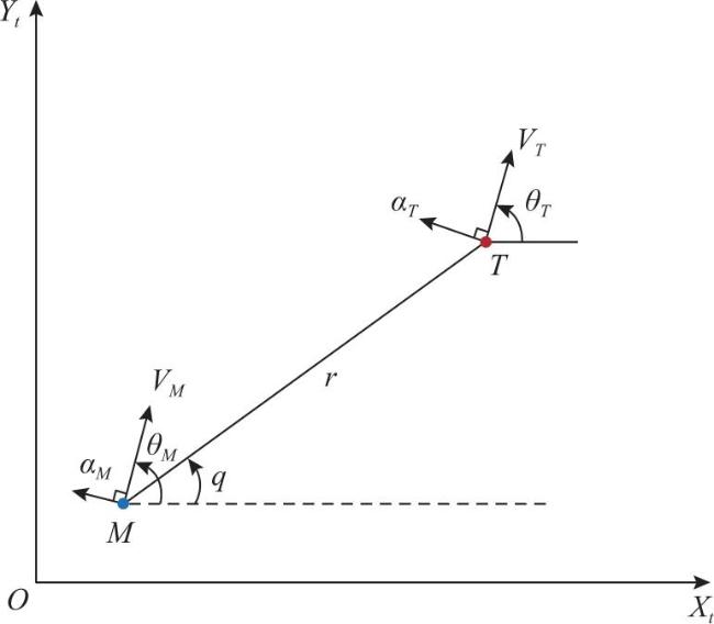
图1 纵向平面交战几何示意图

Fig.1 Planar engagement geometry

其中,X_IOY_I为惯性坐标系,M代表导弹,T代表目标。V_M,V_T分别代表导弹和目标的速度。a_M,a_T分别代表导弹和目标的法向加速度。θ_M,θ_T分别代表导弹和目标的速度倾角。r代表导弹与目标之间的距离。q代表导弹与目标之间的视线角。

根据图1,描述交战几何关系的微分方程可表示为

(1) $\stackrel{\mathit{　}·}{\mathit{r}}$=V_Tcos(θ_T-q)-V_Mcos(θ_M-q)

(2) $\stackrel{\mathit{　}·}{\mathit{q}}$= $\frac{{\mathit{V}}_{\mathit{T}}\mathit{s}\mathit{i}\mathit{n}({\mathit{\theta }}_{\mathit{T}}-\mathit{q})-{\mathit{V}}_{\mathit{M}}\mathit{s}\mathit{i}\mathit{n}({\mathit{\theta }}_{\mathit{M}}-\mathit{q})}{\mathit{r}}$

(3) ${\stackrel{\mathit{　}·}{\mathit{\theta }}}_{\mathit{M}}$= $\frac{{\mathit{a}}_{\mathit{M}}}{{\mathit{V}}_{\mathit{M}}}$

(4) ${\stackrel{\mathit{　}·}{\mathit{\theta }}}_{\mathit{T}}$= $\frac{{\mathit{a}}_{\mathit{T}}}{{\mathit{V}}_{\mathit{T}}}$

对于公式(1)-(4)所示的非线性动力学系统,基于该系统很难求得解析形式的最优制导律。为了应对该问题,传统方法是将式(1)-(4)在小角假设下线性化,并假设目标执行常值机动预测ZEM,基于最优控制理论设计解析制导律^[19]。然而,该设计方法存在缺陷:当高机动目标在执行复杂机动时,其机动形式难以预测,采用常值机动假设预测的ZEM存在较大误差,无法精准补偿目标机动,导致末端需用过载高。

为克服上述问题,本文引入相对参考系进行建模,对目标过载进行实时精确补偿,避免传统方法预测目标未来机动形式失准而带来过补偿或欠补偿导致需用过载增大。

1.2 相对参考系下的运动关系

相对参考系下,导弹与目标间的相对运动关系如图2所示。

显示原图|下载原图ZIP|生成PPT

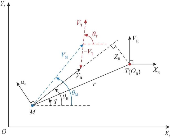
图2 参考系下的相对运动关系

Fig.2 Engagement geometry in reference frame

其中,导弹与目标间的相对速度矢量V_R定义为V_R=V_M-V_T,a_n表示相对法向加速度。由图2中几何关系可知,相对速度V_R和相对速度倾角θ_R为

(5)V_R= $\sqrt{{\mathit{V}}_{\mathit{M}}^{2}+{\mathit{V}}_{\mathit{T}}^{2}-2{\mathit{V}}_{\mathit{M}}{\mathit{V}}_{\mathit{T}}\mathit{c}\mathit{o}\mathit{s}({\mathit{\theta }}_{\mathit{M}}-{\mathit{\theta }}_{\mathit{T}})}$

(6)θ_R=arctan $\left(\frac{\mathit{s}\mathit{i}\mathit{n}{\mathit{\theta }}_{\mathit{M}}-\mathit{K}\mathit{s}\mathit{i}\mathit{n}{\mathit{\theta }}_{\mathit{T}}}{\mathit{c}\mathit{o}\mathit{s}{\mathit{\theta }}_{\mathit{M}}-\mathit{K}\mathit{c}\mathit{o}\mathit{s}{\mathit{\theta }}_{\mathit{T}}}\right)$

式中,K=V_T/V_M,表示目标与导弹的速度大小之比。

相对参考系下的相对运动方程可表示为

(7) $\stackrel{\mathit{　}·}{\mathit{r}}$=-V_Rcos(θ_R-q)

(8) $\stackrel{\mathit{　}·}{\mathit{q}}$= $\frac{-{\mathit{V}}_{\mathit{R}}\mathit{s}\mathit{i}\mathit{n}({\mathit{\theta }}_{\mathit{R}}-\mathit{q})}{\mathit{r}}$

(9) ${\stackrel{\mathit{　}·}{\mathit{\theta }}}_{\mathit{R}}$= $\frac{{\mathit{a}}_{\mathit{n}}}{{\mathit{V}}_{\mathit{R}}}$

(10) ${\stackrel{\mathit{　}·}{\mathit{V}}}_{\mathit{R}}$=f₁(V_R)a_n+f₂(V_R)a_T

式中,

(11)f₁(V_R)=tan(θ_R-θ_M)

(12)

$\begin{array}{c}{\mathit{f}}_{2}\left({\mathit{V}}_{\mathit{R}}\right)=\mathit{t}\mathit{a}\mathit{n}({\mathit{\theta }}_{\mathit{R}}-{\mathit{\theta }}_{\mathit{M}})\mathit{c}\mathit{o}\mathit{s}({\mathit{\theta }}_{\mathit{R}}-{\mathit{\theta }}_{\mathit{T}})-\mathit{s}\mathit{i}\mathit{n}({\mathit{\theta }}_{\mathit{R}}-{\mathit{\theta }}_{\mathit{T}})\end{array}$

(13)a_n=a_Mcos(θ_R-θ_M)-a_Tcos(θ_R-θ_T)

根据文献[11],惯性系下的速度倾角θ_M,θ_T与相对参考系下的相对速度倾角θ_R存在以下关系:

(14)θ_M-θ_R=arccos $\left(\frac{1-{\mathit{K}}^{2}+\frac{{\mathit{V}}_{\mathit{R}}^{2}}{{\mathit{V}}_{\mathit{M}}^{2}}}{\frac{2{\mathit{V}}_{\mathit{R}}}{{\mathit{V}}_{\mathit{M}}}}\right)$

(15)

$\begin{array}{c}{\mathit{\theta }}_{\mathit{T}}-{\mathit{\theta }}_{\mathit{R}}=\mathit{a}\mathit{r}\mathit{c}\mathit{c}\mathit{o}\mathit{s}\left(\frac{1-{\mathit{K}}^{2}+\frac{{\mathit{V}}_{\mathit{R}}^{2}}{{\mathit{V}}_{\mathit{M}}^{2}}}{\frac{2{\mathit{V}}_{\mathit{R}}}{{\mathit{V}}_{\mathit{M}}}}\right)-\mathit{a}\mathit{r}\mathit{c}\mathit{c}\mathit{o}\mathit{s}\left(\frac{1+{\mathit{K}}^{2}-\frac{{\mathit{V}}_{\mathit{R}}^{2}}{{\mathit{V}}_{\mathit{M}}^{2}}}{\frac{2{\mathit{V}}_{\mathit{R}}}{{\mathit{V}}_{\mathit{M}}}}\right)\end{array}$

根据动力学方程(7)-(10)可设计解析形式的最优制导律。

2 最优制导律设计

2.1 均势拦截的必要条件

根据图2中的几何关系,相对参考系下的ZEM可定义为

(16)Z_R=-rsin(θ_R-q)

式(16)的物理意义是,若相对速度V_R的方向不再发生改变,则拦截末端的脱靶量为Z_R。

对式(13)移项可得

(17)a_M= $\frac{1}{\mathit{c}\mathit{o}\mathit{s}({\mathit{\theta }}_{\mathit{R}}-{\mathit{\theta }}_{\mathit{M}})}$a_n+ $\frac{\mathit{c}\mathit{o}\mathit{s}({\mathit{\theta }}_{\mathit{R}}-{\mathit{\theta }}_{\mathit{T}})}{\mathit{c}\mathit{o}\mathit{s}({\mathit{\theta }}_{\mathit{R}}-{\mathit{\theta }}_{\mathit{M}})}$a_T

式(17)表明惯性系下的导弹法向加速度由两部分组成,第一部分用于调节相对速度的方向,第二部分用于抵消目标机动的影响。

对式(17)等式两侧取绝对值有

(18) $\left|{\mathit{a}}_{\mathit{M}}\right|$= $\left|\frac{1}{\mathit{c}\mathit{o}\mathit{s}({\mathit{\theta }}_{\mathit{R}}-{\mathit{\theta }}_{\mathit{M}})}{\mathit{a}}_{\mathit{n}}+\frac{\mathit{c}\mathit{o}\mathit{s}({\mathit{\theta }}_{\mathit{R}}-{\mathit{\theta }}_{\mathit{T}})}{\mathit{c}\mathit{o}\mathit{s}({\mathit{\theta }}_{\mathit{R}}-{\mathit{\theta }}_{\mathit{M}})}{\mathit{a}}_{\mathit{T}}\right|$

根据图2几何关系以及速度关系V_M>V_T,可得如下结论:

(19) $\left|{\mathit{\theta }}_{\mathit{M}}-{\mathit{\theta }}_{\mathit{R}}\right|$≤ $\left|{\mathit{\theta }}_{\mathit{T}}-{\mathit{\theta }}_{\mathit{R}}\right|$

因此,进一步可得

(20) $\left|\frac{\mathit{c}\mathit{o}\mathit{s}({\mathit{\theta }}_{\mathit{R}}-{\mathit{\theta }}_{\mathit{T}})}{\mathit{c}\mathit{o}\mathit{s}({\mathit{\theta }}_{\mathit{R}}-{\mathit{\theta }}_{\mathit{M}})}\right|$≤1

将式(20)代入式(18),并应用三角不等式可得

(21)$\begin{aligned} \left|a_{\mathrm{M}}\right| & \leqslant\left|\frac{1}{\cos \left(\theta_{\mathrm{R}}-\theta_{\mathrm{M}}\right)}\right|\left|a_{n}\right|+\left|\frac{\cos \left(\theta_{\mathrm{R}}-\theta_{\mathrm{T}}\right)}{\cos \left(\theta_{\mathrm{R}}-\theta_{\mathrm{M}}\right)}\right|\left|a_{\mathrm{T}}\right| \\ & \leqslant\left|\frac{1}{\cos \left(\theta_{\mathrm{R}}-\theta_{\mathrm{M}}\right)}\right|\left|a_{n}\right|+\left|a_{\mathrm{T}}\right| \end{aligned}$

根据Z_R的定义和物理意义可知,垂直于相对速度方向的法向加速度a_n用于消除Z_R。当Z_R=0时,即相对参考系下的ZEM已被完全消除,导弹此时已经对准目标,因此a_n=0。此时,式(21)退化为

(22) $\left|{\mathit{a}}_{\mathit{M}}\right|$≤ $\left|{\mathit{a}}_{\mathit{T}}\right|$

由此可知,当Z_R=0时, a_n=0,目标机动将由式(17)中的第二项抵消,导弹的过载比将满足式(22)的约束。因此,在相对参考系下,导弹实现均势过载拦截的必要条件为

(23)Z_R(t_f)=0

若式(23)能在指定时间t_s∈[t₀,t_f]处提前满足,即

(24)Z_R(t_s)=0

则在理想情况下,导弹只需在在t∈[t_s,t_f]内生成应对目标机动的补偿指令即可,且在该段时间内导弹均满足式(22)的约束。因此,导弹的制导律可以分为两阶段进行设计。第一阶段,导弹在最短距离内消除指向误差,收敛至均势拦截约束式(24)。第二阶段,导弹以最小需用过载抵消目标机动和内回路延迟的影响,实现对高机动目标的末端均势拦截。

2.2 制导律设计

在相对参考系下,由式(7)-(10)构建的动力学模型较为复杂,最优制导律的解析求解较为困难。为便于推导求解,对该组动力学约束进行降维处理。

导弹飞行过程中,r随时间单调递减,因此可将式(7)-(10)转换至距离如下表示:

(25) $\frac{\mathit{d}\mathit{q}}{\mathit{d}\mathit{r}}$= $\frac{1}{\mathit{r}}$tan(θ_R-q)

(26) $\frac{\mathit{d}{\mathit{\theta }}_{\mathit{R}}}{\mathit{d}\mathit{r}}$=- $\frac{{\mathit{a}}_{\mathit{n}}}{{\mathit{V}}_{\mathit{R}}^{2}\mathit{c}\mathit{o}\mathit{s}({\mathit{\theta }}_{\mathit{R}}-\mathit{q})}$

(27) $\frac{\mathit{d}{\mathit{V}}_{\mathit{R}}}{\mathit{d}\mathit{r}}$=- $\frac{{\mathit{f}}_{1}\left({\mathit{V}}_{\mathit{R}}\right){\mathit{a}}_{\mathit{n}}+{\mathit{f}}_{2}\left({\mathit{V}}_{\mathit{R}}\right){\mathit{a}}_{\mathit{T}}}{{\mathit{V}}_{\mathit{R}}\mathit{c}\mathit{o}\mathit{s}({\mathit{\theta }}_{\mathit{R}}-\mathit{q})}$

观察式(16)、(25)-(27)可知,Z_R是q,θ_R和r的函数,而实现均势过载拦截的必要条件完全由Z_R决定,因此可将Z_R的动力学作为过程约束,替代式(25)-(26)以实现模型降维。对式(16)关于r求导,并联立式(25)-(26)可得

(28) $\frac{\mathit{d}{\mathit{Z}}_{\mathit{R}}}{\mathit{d}\mathit{r}}$=r

$\frac{{\mathit{a}}_{\mathit{n}}}{{\mathit{V}}_{\mathit{R}}^{2}}$

定义伪控制量u为

(29)u= $\frac{{\mathit{a}}_{\mathit{n}}}{{\mathit{V}}_{\mathit{R}}^{2}}$

则式(28)可表示为

(30) $\frac{\mathit{d}{\mathit{Z}}_{\mathit{R}}}{\mathit{d}\mathit{r}}$=ru

由于式(30)不显含相对速度V_R,因此V_R的动力学不影响Z_R的动力学,则动力学约束式(27)可忽略。在距离域下,均势过载拦截必要条件式(24)可转换为

(31)Z_R(r_s)=0

式中,r_s为t_s时刻,导弹与目标间的距离。

第一阶段制导律的目的是让导弹在最短距离范围内消除指向误差,因此第一阶段的最优控制问题可构建为如下形式:

(32)

$\begin{array}{l}\underset{\mathit{u}}{\mathit{m}\mathit{i}\mathit{n}}\mathit{J}={\int }_{{\mathit{r}}_{\mathit{s}}}^{\mathit{r}}\mathit{d}\mathit{l}\\ \mathit{s}.\mathit{t}.\frac{\mathit{d}{\mathit{Z}}_{\mathit{R}}}{\mathit{d}\mathit{r}}=\mathit{r}\mathit{u}\\ {\mathit{Z}}_{\mathit{R}}\left({\mathit{r}}_{\mathit{s}}\right)=0\\ \left|\mathit{u}\right|\le {\mathit{u}}_{\mathit{m}\mathit{a}\mathit{x}\mathit{ }}\end{array}$

该最优控制问题的哈密顿函数为

(33)H₁=1+λ₁ru

根据庞特里亚金极小值原理,使哈密顿函数H₁取极小值的控制量u是该最优控制问题的解。在导弹飞行过程中,r始终为正值,则最优控制解可表示为

(34)u^*=-u_maxsign(λ₁)

式中,sign(·)表示符号函数。该最优控制问题的协状态方程可表示为

(35)

$\stackrel{\mathit{　}·}{\mathit{\lambda }}$

₁=- $\frac{\partial {\mathit{H}}_{1}}{\partial {\mathit{Z}}_{\mathit{R}}}$=0

这表明协状态λ₁是常量。对式(30)两侧同时积分并代入式(34)可求得

(36)Z_R=- $\frac{1}{2}$u_maxsign(λ₁)(r²- ${\mathit{r}}_{\mathit{s}}^{2}$)

由于

$\frac{1}{2}$

u_max(r²-

${\mathit{r}}_{\mathit{s}}^{2}$

)>0恒成立,因此有

(37)sign(Z_R)=-sign(λ₁)

则最优控制解可表示为

(38)u^*=u_maxsign(Z_R)

实际应用中,执行机构偏转能力限制的是导弹的法向过载能力,因此,第一阶段最优相对法向加速度可表示为

(39) ${\mathit{a}}_{\mathit{n}}^{\mathit{*}}$=a_Mmaxsign(Z_R)

实际应用中,Z_R通常难以直接测量获得。联立式(8)和(16)可得

(40)Z_R= $\frac{\stackrel{\mathit{　}·}{\mathit{q}}{\mathit{r}}^{2}}{{\mathit{V}}_{\mathit{R}}}$

式中,视线角速率

$\stackrel{\mathit{　}·}{\mathit{q}}$

和距离r可直接通过导引头测量获得。相对速度大小V_R可通过惯导信息和导引头测量信息滤波得出。

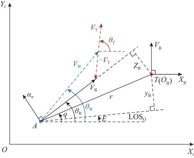
第二阶段,即t∈[t_s,t_f]内,以最小需用过载抵消目标机动和内回路延迟的影响。由于引入了内回路延迟,若在相对参考系下直接设计第二阶段最优制导律将难以求得解析解。一般认为,固定视线方向之后,视线角的变化范围在±15°之内时,线性化误差较小,可被忽略,小角假设成立^[20]。由式(31)可知,当第一阶段制导结束时,指向误差已被消除,视线角的变化幅度很小,满足小角假设。因此可对图2所示的相对参考系进行线性化,如图3所示。

显示原图|下载原图ZIP|生成PPT

图3 线性化相对参考坐标系

Fig.3 Linearized reference frame

其中,LOS₀表示第一阶段制导结束时,目标指向导弹的视线方向,此时,(θ_R-q)=0。y_R表示侧向偏差,其动力学可表示为

(41)

$\stackrel{\mathit{　}··}{\mathit{y}}$

_R=-a_ncos(q-ε)

在小角假设下,(q-ε)很小,即cos(q-ε)≈1,则y_R的动力学可进一步表示为

(42)

$\stackrel{\mathit{　}··}{\mathit{y}}$

_R=-a_n

根据式(17)和图2,导弹执行机构动力学、目标执行机构动力学、相对法向加速度动力学存在如下关系:

(43) ${\stackrel{\mathit{　}·}{\mathit{a}}}_{\mathit{n}}$= ${\stackrel{\mathit{　}·}{\mathit{a}}}_{\mathit{M}}$- ${\stackrel{\mathit{　}·}{\mathit{a}}}_{\mathit{T}}$

式(43)表明,导弹和目标的执行机构动力学可转换至相对参考坐标系下进行补偿。假设导弹和目标的执行机构动力学分别为

(44) $\frac{{\mathit{a}}_{\mathit{M}\mathit{L}}}{{\mathit{a}}_{\mathit{M}}}$= $\frac{1}{{\mathit{T}}_{1}\mathit{s}+1}$

和

(45) $\frac{{\mathit{a}}_{\mathit{T}\mathit{L}}}{{\mathit{a}}_{\mathit{T}}}$= $\frac{1}{{\mathit{T}}_{2}\mathit{s}+1}$

则相对法向加速度的动力学可表示为

(46)

$\begin{array}{l}\frac{{\mathit{a}}_{\mathit{n}\mathit{L}}}{{\mathit{a}}_{\mathit{n}}}=\frac{1}{{\mathit{T}}_{1}\mathit{s}+1}-\frac{1}{{\mathit{T}}_{2}\mathit{s}+1}\\ =\frac{\mathit{K}\mathit{s}}{\mathit{M}{\mathit{s}}^{2}+\mathit{N}\mathit{s}+1}\end{array}$

式中,K=T₂-T₁, M=T₁T₂, N=T₁+T₂。显然,a_n的动力学特性为二阶,对其求反拉普拉斯变换可得其时域表达式为

(47)M ${\stackrel{\mathit{　}··}{\mathit{a}}}_{\mathit{n}\mathit{L}}$+N

$\stackrel{\mathit{　}·}{\mathit{a}}$

_nL+a_nL=K

$\stackrel{\mathit{　}·}{\mathit{a}}$

为了消去输入导数项,定义新状态:

(48)ξ= $\stackrel{\mathit{　}·}{\mathit{a}}$_nL- $\frac{\mathit{K}}{\mathit{M}}$a_n

则

$\stackrel{\mathit{　}·}{\mathit{a}}$

_nL可表示为

(49)

$\stackrel{\mathit{　}·}{\mathit{a}}$

_nL=ξ+ $\frac{\mathit{K}}{\mathit{M}}$a_n

ξ的动力学表示为

(50) $\stackrel{\mathit{　}·}{\mathit{\xi }}$= $\stackrel{\mathit{　}··}{\mathit{a}}$_nL- $\frac{\mathit{K}}{\mathit{M}}\stackrel{\mathit{　}·}{\mathit{a}}$_n

联立式(47)可得

(51) $\stackrel{\mathit{　}·}{\mathit{\xi }}$=- $\frac{\mathit{N}}{\mathit{M}}$ξ- $\frac{1}{\mathit{M}}$a_nL- $\frac{\mathit{N}\mathit{K}}{{\mathit{M}}^{2}}$a_n

则描述导弹与目标间相对运动关系的状态方程可构建为

(52) $\left[\begin{array}{l}\stackrel{\mathit{　}·}{\mathit{y}}{\mathit{ }}_{\mathit{R}}\\ \stackrel{\mathit{　}··}{\mathit{y}}{\mathit{ }}_{\mathit{R}}\\ \stackrel{\mathit{　}·}{\mathit{a}}{\mathit{ }}_{\mathit{n}\mathit{L}}\\ \stackrel{\mathit{　}·}{\mathit{\xi }}\end{array}\right]$= $\left[\begin{array}{llll}0& 1& 0& 0\\ 0& 0& -1& 0\\ 0& 0& 0& 1\\ 0& 0& -\frac{1}{\mathit{M}}& -\frac{\mathit{N}}{\mathit{M}}\end{array}\right]\left[\begin{array}{l}{\mathit{y}}_{\mathit{R}}\\ \stackrel{\mathit{　}·}{\mathit{y}}{\mathit{ }}_{\mathit{R}}\\ {\mathit{a}}_{\mathit{n}\mathit{L}}\\ \mathit{\xi }\end{array}\right]$+ $\left[\begin{array}{l}0\\ 0\\ \frac{\mathit{K}}{\mathit{M}}\\ -\frac{\mathit{N}\mathit{K}}{{\mathit{M}}^{2}}\end{array}\right]$a_n

该状态方程可表示为

(53) $\stackrel{\mathit{　}·}{\mathit{X}}$=FX+GU

其中,F=

$\left[\begin{array}{llll}0& 1& 0& 0\\ 0& 0& -1& 0\\ 0& 0& 0& 1\\ 0& 0& -\frac{1}{\mathit{M}}& -\frac{\mathit{N}}{\mathit{M}}\end{array}\right]$

,G=

$\left[\begin{array}{l}0\\ 0\\ \frac{\mathit{K}}{\mathit{M}}\\ -\frac{\mathit{N}\mathit{K}}{{\mathit{M}}^{2}}\end{array}\right]$

,U=a_n。

在线性化相对参考系下,导弹实现小过载比拦截的必要条件转化为

(54)y_R(t_f)=0

根据式(42)可知,第二阶段的动力学方程是线性的,无需转换至距离域下进行降维处理。因此,可在时域下构建第二阶段的最优控制问题为

(55)

$\begin{array}{l}\underset{{\mathit{a}}_{\mathit{n}}}{\mathit{m}\mathit{i}\mathit{n}}\mathit{J}={\int }_{\mathit{t}}^{{\mathit{t}}_{\mathit{f}}}{\mathit{a}}_{\mathit{n}}^{2}\mathit{d}\mathit{t}\\ \mathit{s}.\mathit{t}.\mathit{ }{\mathit{y}}_{\mathit{R}}\left({\mathit{t}}_{\mathit{f}}\right)=0\end{array}$

根据现代控制理论^[8],状态空间表达式(52)的解为

(56)

$\mathit{X}\left({\mathit{t}}_{\mathit{f}}\right)=\mathit{\Phi }({\mathit{t}}_{\mathit{f}}-\mathit{t})\mathit{X}\left(\mathit{t}\right)+{\int }_{\mathit{t}}^{{\mathit{t}}_{\mathit{f}}}\mathit{\Phi }({\mathit{t}}_{\mathit{f}}-\mathit{\tau })\mathit{G}\left(\mathit{\tau }\right)\mathit{U}\left(\mathit{\tau }\right)\mathit{d}\mathit{\tau }$

式中,Φ表示状态转移矩阵,其表达式为

(57)Φ(t)=L^-1[(sI-F)^-1]

其中,L^-1表示拉普拉斯逆变换。联立式(52)与(57)可得

(58)Φ(t)= $\left[\begin{array}{llll}1& \mathit{t}& -{\mathit{I}}_{3}\left(\mathit{t}\right)& -{\mathit{I}}_{4}\left(\mathit{t}\right)\\ 0& 1& -{\mathit{I}}_{1}\left(\mathit{t}\right)& -{\mathit{I}}_{2}\left(\mathit{t}\right)\\ 0& 0& {\mathit{\varphi }}_{11}\left(\mathit{t}\right)& {\mathit{\varphi }}_{12}\left(\mathit{t}\right)\\ 0& 0& {\mathit{\varphi }}_{21}\left(\mathit{t}\right)& {\mathit{\varphi }}_{22}\left(\mathit{t}\right)\end{array}\right]$

式中,

(59)φ₁₁(t)= $\frac{{\mathit{T}}_{1}{\mathit{e}}^{-\mathit{t}/{\mathit{T}}_{1}}-{\mathit{T}}_{2}{\mathit{e}}^{-\mathit{t}/{\mathit{T}}_{2}}}{{\mathit{T}}_{1}-{\mathit{T}}_{2}}$

(60)φ₁₂(t)= $\frac{{\mathit{T}}_{1}{\mathit{T}}_{2}({\mathit{e}}^{-\mathit{t}/{\mathit{T}}_{1}}-{\mathit{e}}^{-\mathit{t}/{\mathit{T}}_{2}})}{{\mathit{T}}_{1}-{\mathit{T}}_{2}}$

(61)φ₂₁(t)= $\frac{{\mathit{e}}^{-\mathit{t}/{\mathit{T}}_{2}}-{\mathit{e}}^{-\mathit{t}/{\mathit{T}}_{1}}}{{\mathit{T}}_{1}-{\mathit{T}}_{2}}$

(62)φ₂₂(t)= $\frac{{\mathit{T}}_{2}{\mathit{e}}^{-\mathit{t}/{\mathit{T}}_{2}}-{\mathit{T}}_{1}{\mathit{e}}^{-\mathit{t}/{\mathit{T}}_{1}}}{{\mathit{T}}_{1}-{\mathit{T}}_{2}}$

(63)I₁(t)= $\frac{{\mathit{T}}_{1}^{2}(1-{\mathit{e}}^{-\mathit{t}/{\mathit{T}}_{1}})-{\mathit{T}}_{2}^{2}(1-{\mathit{e}}^{-\mathit{t}/{\mathit{T}}_{2}})}{{\mathit{T}}_{1}-{\mathit{T}}_{2}}$

(64)I₂(t)= $\frac{{\mathit{T}}_{1}^{2}{\mathit{T}}_{2}(1-{\mathit{e}}^{-\mathit{t}/{\mathit{T}}_{1}})-{\mathit{T}}_{1}{\mathit{T}}_{2}^{2}(1-{\mathit{e}}^{-\mathit{t}/{\mathit{T}}_{2}})}{{\mathit{T}}_{1}-{\mathit{T}}_{2}}$

(65)I₃(t)=(T₁+T₂)t-(${\mathit{T}}_{1}^{2}$+T₁T₂+ ${\mathit{T}}_{2}^{2}$)+ $\frac{{\mathit{T}}_{1}^{3}{\mathit{e}}^{-\mathit{t}/{\mathit{T}}_{1}}-{\mathit{T}}_{2}^{3}{\mathit{e}}^{-\mathit{t}/{\mathit{T}}_{2}}}{{\mathit{T}}_{1}-{\mathit{T}}_{2}}$

(66)I₄(t)=T₁T₂[t-(T₁+T₂)]+ $\frac{{\mathit{T}}_{1}^{3}{\mathit{T}}_{2}{\mathit{e}}^{-\mathit{t}/{\mathit{T}}_{1}}-{\mathit{T}}_{1}{\mathit{T}}_{2}^{3}{\mathit{e}}^{-\mathit{t}/{\mathit{T}}_{2}}}{{\mathit{T}}_{1}-{\mathit{T}}_{2}}$

联立式(56)与(58)并提取状态空间表达式解空间中y_R的解,有

(67)

${\mathit{y}}_{\mathit{R}}\left({\mathit{t}}_{\mathit{f}}\right)={\mathit{f}}_{1}({\mathit{t}}_{\mathit{f}}-\mathit{t})-{\int }_{\mathit{t}}^{{\mathit{t}}_{\mathit{f}}}{\mathit{h}}_{1}({\mathit{t}}_{\mathit{f}}-\mathit{\tau }){\mathit{a}}_{\mathit{n}}\left(\mathit{\tau }\right)\mathit{d}\mathit{\tau }$

式中,

(68)f₁(t_f-t)=y_R(t)+ $\stackrel{\mathit{　}·}{\mathit{y}}$_R(t)t_go-I₃(t_go)a_nL(t)-I₄(t_go)ξ(t)

(69)

$\begin{array}{c}{\mathit{I}}_{3}({\mathit{t}}_{\mathit{f}}-\mathit{t})=({\mathit{T}}_{1}+{\mathit{T}}_{2}){\mathit{t}}_{\mathit{g}\mathit{o}}-({\mathit{T}}_{1}^{2}+{\mathit{T}}_{1}{\mathit{T}}_{2}+{\mathit{T}}_{2}^{2})+\frac{{\mathit{T}}_{1}^{3}{\mathit{e}}^{-{\mathit{t}}_{\mathit{g}\mathit{o}}/{\mathit{T}}_{1}}-{\mathit{T}}_{2}^{3}{\mathit{e}}^{-{\mathit{t}}_{\mathit{g}\mathit{o}}/{\mathit{T}}_{2}}}{{\mathit{T}}_{1}-{\mathit{T}}_{2}}\end{array}$

(70)

$\begin{array}{c}{\mathit{I}}_{4}({\mathit{t}}_{\mathit{f}}-\mathit{t})={\mathit{T}}_{1}{\mathit{T}}_{2}[{\mathit{t}}_{\mathit{g}\mathit{o}}-({\mathit{T}}_{1}+{\mathit{T}}_{2}\left)\right]+\frac{{\mathit{T}}_{1}^{3}{\mathit{T}}_{2}{\mathit{e}}^{-{\mathit{t}}_{\mathit{g}\mathit{o}}/{\mathit{T}}_{1}}-{\mathit{T}}_{1}{\mathit{T}}_{2}^{3}{\mathit{e}}^{-{\mathit{t}}_{\mathit{g}\mathit{o}}/{\mathit{T}}_{2}}}{{\mathit{T}}_{1}-{\mathit{T}}_{2}}\end{array}$

(71)h₁(t_f-t)=(T₁-T₂)-T₁e^-t_go/T₁+T₂e^-t_go/T₂

式中,t_go=t_f-t表示导弹与目标之间的剩余飞行时间,可由下式估计得到

(72)t_go=- $\frac{\mathit{r}}{\stackrel{\mathit{　}·}{\mathit{r}}}$

代入式(54)中的终端约束条件,有

(73)

${\mathit{f}}_{1}({\mathit{t}}_{\mathit{f}}-\mathit{t})={\int }_{\mathit{t}}^{{\mathit{t}}_{\mathit{f}}}{\mathit{h}}_{1}({\mathit{t}}_{\mathit{f}}-\mathit{\lambda }){\mathit{a}}_{\mathit{n}}\left(\mathit{\tau }\right)\mathit{d}\mathit{\tau }$

对式(73)应用柯西-施瓦茨不等式^[21],有

(74)

$\mathit{f}{\mathit{ }}_{1}^{2}({\mathit{t}}_{\mathit{f}}-\mathit{t})\le {\int }_{\mathit{t}}^{{\mathit{t}}_{\mathit{f}}}{\mathit{h}}_{1}^{2}({\mathit{t}}_{\mathit{f}}-\mathit{\tau })\mathit{d}\mathit{\tau }{\int }_{\mathit{t}}^{{\mathit{t}}_{\mathit{f}}}{\mathit{a}}_{\mathit{n}}^{2}\left(\mathit{\tau }\right)\mathit{d}\mathit{\tau }$

移项可得

(75)

${\int }_{\mathit{t}}^{{\mathit{t}}_{\mathit{f}}}{\mathit{a}}_{\mathit{n}}^{2}\left(\mathit{\tau }\right)\mathit{d}\mathit{\tau }\ge \frac{\mathit{f}{\mathit{ }}_{1}^{2}({\mathit{t}}_{\mathit{f}}-\mathit{t})}{{\int }_{\mathit{t}}^{{\mathit{t}}_{\mathit{f}}}{\mathit{h}}_{1}^{2}({\mathit{t}}_{\mathit{f}}-\mathit{\tau })\mathit{d}\mathit{\tau }}$

式(75)表明,当不等式等号成立时,不等式左侧取得最小值。根据柯西-施瓦茨不等式,等号成立的条件为

(76)a_n(τ)=kh₁(t_f-τ)

将上式两侧同乘h₁(t_f-τ)并在[t,t_f]内积分,可得

(77)

$\mathit{k}=\frac{{\mathit{f}}_{1}({\mathit{t}}_{\mathit{f}}-\mathit{t})}{{\int }_{\mathit{t}}^{{\mathit{t}}_{\mathit{f}}}{\mathit{h}}_{1}^{2}({\mathit{t}}_{\mathit{f}}-\mathit{\tau })\mathit{d}\mathit{\tau }}$

式(77)中积分项的积分结果为

(78)

$\begin{array}{l}{\int }_{\mathit{t}}^{{\mathit{t}}_{\mathit{f}}}{\mathit{h}}_{1}^{2}({\mathit{t}}_{\mathit{f}}-\mathit{\tau })\mathit{d}\mathit{\tau }=({\mathit{T}}_{1}-{\mathit{T}}_{2}{)}^{2}{\mathit{t}}_{\mathit{g}\mathit{o}}+\frac{{\mathit{T}}_{1}^{3}}{2}(1-{\mathit{e}}^{-2{\mathit{t}}_{\mathit{g}\mathit{o}}/{\mathit{T}}_{1}})\\ +\frac{{\mathit{T}}_{2}^{3}}{2}(1-{\mathit{e}}^{-2{\mathit{t}}_{\mathit{g}\mathit{o}}/{\mathit{T}}_{2}})+2({\mathit{T}}_{1}-{\mathit{T}}_{2}){\mathit{T}}_{1}^{2}({\mathit{e}}^{-{\mathit{t}}_{\mathit{g}\mathit{o}}/{\mathit{T}}_{1}}-1)\\ -2({\mathit{T}}_{1}-{\mathit{T}}_{2}){\mathit{T}}_{2}^{2}({\mathit{e}}^{-{\mathit{t}}_{\mathit{g}\mathit{o}}/{\mathit{T}}_{2}}-1)+\frac{2{\mathit{T}}_{1}^{2}{\mathit{T}}_{2}^{2}}{{\mathit{T}}_{1}+{\mathit{T}}_{2}}({\mathit{e}}^{-{\mathit{t}}_{\mathit{g}\mathit{o}}({\mathit{T}}_{1}+{\mathit{T}}_{2})/({\mathit{T}}_{1}{\mathit{T}}_{2})}-1)\end{array}$

联立式(68)-(71)和(78),可得第二阶段最优制导律为

(79)

${\mathit{a}}_{\mathit{n}}^{\mathit{*}}=\left[\frac{{\mathit{f}}_{1}({\mathit{t}}_{\mathit{f}}-\mathit{t})}{{\int }_{\mathit{t}}^{{\mathit{t}}_{\mathit{f}}}{\mathit{h}}_{1}^{2}({\mathit{t}}_{\mathit{f}}-\mathit{\tau })\mathit{d}\mathit{\tau }}\right]{\mathit{h}}_{1}({\mathit{t}}_{\mathit{f}}-\mathit{t})$

根据文献[21],可得如下关系:

(80)y_R(t)+ ${\stackrel{\mathit{　}·}{\mathit{y}}}_{\mathit{R}}$(t)t_go=- $\stackrel{\mathit{　}·}{\mathit{r}}\stackrel{\mathit{　}·}{\mathit{q}}{\mathit{t}}_{\mathit{g}\mathit{o}}^{2}$

联立式(7),(72),(80)可得

(81)y_R(t)+ ${\stackrel{\mathit{　}·}{\mathit{y}}}_{\mathit{R}}$(t)t_go= $\frac{\stackrel{\mathit{　}·}{\mathit{q}}{\mathit{r}}_{}^{2}}{{\mathit{V}}_{\mathit{R}}\mathit{c}\mathit{o}\mathit{s}({\mathit{\theta }}_{\mathit{R}}-\mathit{q})}$

由于第一阶段制导结束时,(θ_R-q)已收敛至0附近,因此cos(θ_R-q)≈1。则根据式(40)可知,式(68)可进一步表示为

(82)f₁(t_f-t)=Z_R(t)-I₃(t_go)a_nL(t)-I₄(t_go)ξ(t)

式中,相对法向加速度反馈a_nL可通过加速度计测量并结合式(17)计算获取。

注 1:状态ξ的值可通过非线性最速跟踪微分器进行估计^[22]。

设非线性最速跟踪微分器的状态为

(83)

$\left\{\begin{array}{l}{\mathit{z}}_{1}={\mathit{a}}_{\mathit{n}\mathit{L}}\\ {\mathit{z}}_{2}=\stackrel{\mathit{　}·}{\mathit{a}}{\mathit{ }}_{\mathit{n}\mathit{L}}\end{array}\right.$

则其动力学方程为

(84)

$\left\{\begin{array}{l}\stackrel{\mathit{　}·}{\mathit{z}}{\mathit{ }}_{1}={\mathit{z}}_{2}\\ \stackrel{\mathit{　}·}{\mathit{z}}{\mathit{ }}_{2}=\mathit{g}({\mathit{z}}_{1}-{\mathit{a}}_{\mathit{n}\mathit{L}},{\mathit{z}}_{2},\mathit{l},\mathit{h})\end{array}\right.$

式中,g(·)为跟踪微分器控制律,其表达式为

(85)g(z₁-a_nL,z₂,l,h)= $\left\{\begin{array}{l}-\mathit{l}·\frac{\mathit{a}}{\mathit{d}},\mathit{ }\left|\mathit{a}\right|\le \mathit{d}\\ -\mathit{l}·\mathit{s}\mathit{i}\mathit{g}\mathit{n}\left(\mathit{a}\right),\mathit{ }\left|\mathit{a}\right|\mathit{d}\end{array}\right.$

其中,

(86)d=lh²

(87) a₀=hz₂

(88)y=z₁-a_nL+a₀

(89)a₁= $\sqrt{\mathit{d}(\mathit{d}+8\left|\mathit{y}\right|)}$

(90)a₂=a₀+ $\frac{\mathit{s}\mathit{i}\mathit{g}\mathit{n}\left(\mathit{y}\right)({\mathit{a}}_{1}-\mathit{d})}{2}$

(91)s_y= $\frac{\mathit{s}\mathit{i}\mathit{g}\mathit{n}(\mathit{y}+\mathit{d})-\mathit{s}\mathit{i}\mathit{g}\mathit{n}(\mathit{y}-\mathit{d})}{2}$

(92)a=(a₀+y-a₂)s_y+a₂

l为跟踪微分器的快速因子,决定跟踪速度,l越大跟踪越快但噪声放大越明显。h为跟踪微分器的滤波因子,h越大输出越平滑但相位滞后也相应增加。

根据式(84)和(85),ξ的估计值如下式所示

(93) $\hat{\mathit{\xi }}$=z₂- $\frac{\mathit{K}}{\mathit{M}}$a_n

结合式(39)和(79),导弹最优相对法向加速度指令可表示为

(94)

${\mathit{a}}_{\mathit{n}}^{\mathit{*}}=\left\{\begin{array}{ll}{{\mathit{a}}_{\mathit{M}}}_{\mathit{m}\mathit{a}\mathit{x}}\mathit{s}\mathit{i}\mathit{g}\mathit{n}\left({\mathit{Z}}_{\mathit{R}}\right),& \mathit{r}{\mathit{r}}_{\mathit{s}}\\ \left[\frac{{\mathit{f}}_{1}({\mathit{t}}_{\mathit{f}}-\mathit{t})}{{\int }_{\mathit{t}}^{{\mathit{t}}_{\mathit{f}}}{\mathit{h}}_{1}^{2}({\mathit{t}}_{\mathit{f}}-\mathit{\tau })\mathit{d}\mathit{\tau }}\right]{\mathit{h}}_{1}({\mathit{t}}_{\mathit{f}}-\mathit{t}),& \mathit{r}\ge {\mathit{r}}_{\mathit{s}}\end{array}\right.$

联立式(17)与式(94),惯性系下可直接应用的最优制导律可表示为

(95) ${\mathit{a}}_{\mathit{M}}^{\mathit{*}}$= $\frac{1}{\mathit{c}\mathit{o}\mathit{s}({\mathit{\theta }}_{\mathit{R}}-{\mathit{\theta }}_{\mathit{M}})}{\mathit{a}}_{\mathit{n}}^{\mathit{*}}$+ $\frac{\mathit{c}\mathit{o}\mathit{s}({\mathit{\theta }}_{\mathit{R}}-{\mathit{\theta }}_{\mathit{T}})}{\mathit{c}\mathit{o}\mathit{s}({\mathit{\theta }}_{\mathit{R}}-{\mathit{\theta }}_{\mathit{M}})}$a_T

注2:实际应用制导律(95)时,无需计算出r_s的具体数值。根据式(40)实时计算Z_R即可。当Z_R满足式(31)的约束条件,即达到Z_R=0附近的邻域后,切换至第二阶段制导律,且制导律一旦进入第二阶段将一直保持在该阶段,即制导律在拦截过程中仅切换一次。因此,该制导律闭环稳定,不会失稳,且无滞环或死区现象。目标的执行机构动力学时间常数T₂可通过改进多模型算法进行实时辨识获取^[23]。

3 仿真验证

本章通过数学仿真对第2节设计的最优制导律进行验证。首先,在目标执行bang-bang机动的条件下,验证导弹在不同初始速度倾角下对目标的拦截效果。随后,在不同误差水平下,验证目标执行机构时间常数辨识误差对制导律性能的影响。然后,将所提制导律与APNG、及文献[11]提出的增强型理想比例导引律Augmented Ideal Proportional Navigation Guidance,AIPNG),及文献[8]提出的最优制导律(Optimal Guidance Law,OGL)进行对比,验证本文所提制导律的优越性。

仿真相关初始条件设定如表1所示。

表1 仿真初始条件

Table 1 Initial conditions of simulation

初始状态量	数值
导弹初始位置(x_M0,y_M0)/m	(0,3000)
目标初始位置(x_T0,y_T0)/m	(12000,3000)
导弹初始速度倾角θ_M0/(°)	10,20,30
目标初始速度倾角θ_T0/(°)	180
导弹速度V_M/(m·s^-1)	600
目标速度V_T/(m·s^-1)	500

目标执行如下所示的bang-bang机动,其机动形式为

(96)a_T= $\left\{\begin{array}{ll}0,& \mathit{r}8000\mathit{m}\\ {\mathit{a}}_{\mathit{T}\mathit{m}\mathit{a}\mathit{x}},& 4000\mathit{m}\le \mathit{r}\le 8000\mathit{m}\\ -{\mathit{a}}_{\mathit{T}\mathit{m}\mathit{a}\mathit{x}},& \mathit{r}4000\mathit{m}\end{array}\right.$

目标最大法向加速度设定为a_T_max=100m/s²。导弹最大法向加速度设定为a_M_max=110m/s²,仅比目标最大法向加速度高出10%。式(44)-(45)所示的导弹和目标的执行机构动力学时间常数分别设定为T₁=0.4s,T₂=0.2s。

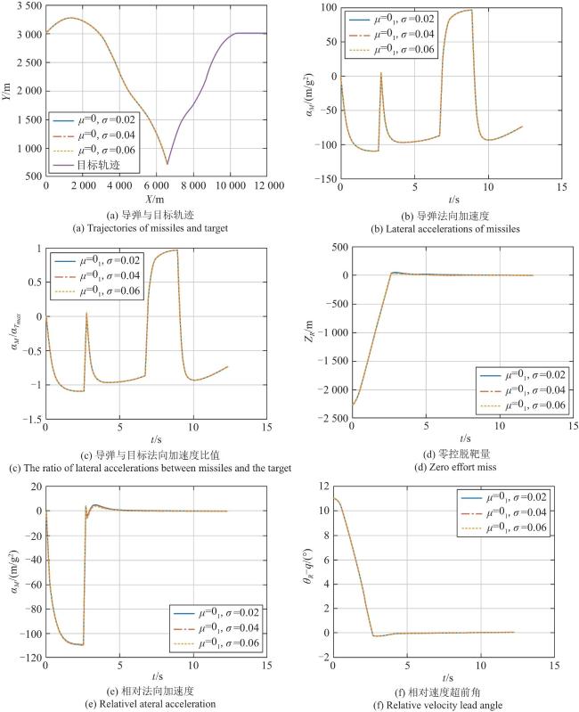
仿真结果如图4所示。

显示原图|下载原图ZIP|生成PPT

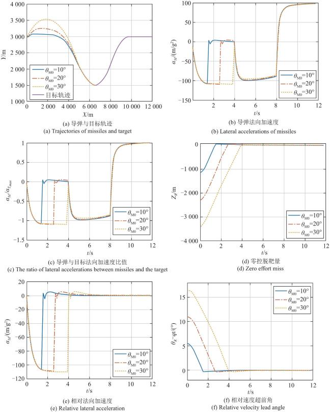
图4 拦截bang-bang机动目标的仿真结果

Fig.4 Simulation results of intercepting a bang-bang maneuvering target

观察仿真结果,图4(a)表明在导弹初始速度倾角分别为10°,20°,30°的条件下,均能精准拦截执行bang-bang机动的目标。观察图4(b)-图4(e)可知,在第一阶段,导弹执行较大机动以迅速消除初始偏差,使ZEM和相对速度超前角(θ_R-q)在最短距离内收敛至0附近较小值,因此相对法向加速度a_n较大,弹目过载比比值较高。在第二阶段,由于ZEM和相对速度超前角(θ_R-q)已收敛至0附近较小值并保持,因此相对法向加速度a_n保持在0附近,此时导弹的法向加速度主要用来抵消目标机动和内回路延迟的影响,该阶段内导弹与目标的法向过载比值始终小于1,满足式(19)的过载比约束。

内回路的参数辨识主要指目标执行机构时间常数T₂的辨识,为了验证时间常数T₂的辨识误差对制导律性能的影响,对T₂施加高斯随机扰动,实际辨识值可表示为

(97)T₂_i=T₂+d

式中,高斯随机扰动d~N(μ,σ²),T₂为目标执行机构时间常数真实值,T_2i为目标执行机构时间常数辨识值。当高斯随机扰动分别服从d~N(0,0.02²), d~N(0,0.04²),d~N(0,0.06²)时,在表1的初始条件下进行仿真,导弹初始速度倾角θ_M0设定为20°,仿真结果如图5所示。

显示原图|下载原图ZIP|生成PPT

图5 不同辨识误差下的仿真结果

Fig.5 Simulation results under different identification errors

仿真结果表明,当目标执行机构动力学时间常数辨识误差分别服从d~N(0,0.02²), d~N(0,0.04²),d~N(0,0.06²)时,导弹均能精准拦截目标,ZEM和相对法向加速度均能在第二阶段收敛至0,实现均势过载拦截。因此,本文所提制导律鲁棒性较强,对目标执行机构动力学时间常数辨识误差不敏感。

为验证辨识误差多大时方法仍有效,取辨识误差为10%,20%,30%,40%,50%,60%,分别进行10000组蒙特卡洛仿真,并绘制脱靶量分布图,结果如图6所示。

显示原图|下载原图ZIP|生成PPT

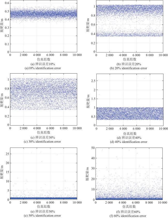
图6 不同辨识误差下的脱靶量

Fig.6 Miss distance under different identification errors

设r<1m为命中条件,则辨识误差为10%,20%,30%,40%,50%,60%时的命中率统计如表2所示。

表2 不同辨识误差下的命中率

Table 2 Hit probability under different identification errors

辨识误差水平	命中率
10%	100%
20%	97.43%
30%	96.36%
40%	94.15%
50%	91.07%
60%	60.43%

图6和表2表明,当辨识误差水平在50%以内时,命中率能够保持在90%以上,当辨识误差水平在30%以内时,命中率能够保持在95%以上,所提制导律仍然有较好性能。而当辨识误差水平达到60%时,命中率急剧下降到60.43%,此时制导律性能难以满足作战需求。

为了进一步说明最优小过载比制导律的优越性,将该制导律与APNG、AIPNG、OGL在表1所示的初始条件下进行对比。对比仿真中,目标的bang-bang机动形式为

(98)a_T= $\left\{\begin{array}{ll}0,& \mathit{r}9000\mathit{m}\\ {\mathit{a}}_{\mathit{T}\mathit{m}\mathit{a}\mathit{x}},& 5000\mathit{m}\mathit{r}\le 9000\mathit{m}\\ -{\mathit{a}}_{\mathit{T}\mathit{m}\mathit{a}\mathit{x}},& 3000\mathit{m}\mathit{r}\le 5000\mathit{m}\\ {\mathit{a}}_{\mathit{T}\mathit{m}\mathit{a}\mathit{x}},& \mathit{r}\le 3000\mathit{m}\end{array}\right.$

APNG的表达式为^[8]

(99)a_APNG= $\frac{\left({\mathit{N}}_{\mathit{A}\mathit{P}\mathit{N}\mathit{G}}{\mathit{V}}_{\mathit{c}}\stackrel{\mathit{　}·}{\mathit{q}}+\frac{{\mathit{N}}_{\mathit{A}\mathit{P}\mathit{N}\mathit{G}}}{2}{\mathit{a}}_{\mathit{T}}\right)}{\mathit{c}\mathit{o}\mathit{s}({\mathit{\theta }}_{\mathit{M}}-\mathit{q})}$

AIPNG的表达式为^[11]

(100)a_AIPNG= $\frac{{\mathit{N}}_{\mathit{A}\mathit{I}\mathit{P}\mathit{N}\mathit{G}}{\mathit{V}}_{\mathit{R}}\stackrel{\mathit{　}·}{\mathit{q}}}{\mathit{c}\mathit{o}\mathit{s}({\mathit{\theta }}_{\mathit{R}}-{\mathit{\theta }}_{\mathit{M}})}$+ $\frac{\mathit{c}\mathit{o}\mathit{s}({\mathit{\theta }}_{\mathit{R}}-{\mathit{\theta }}_{\mathit{T}})}{\mathit{c}\mathit{o}\mathit{s}({\mathit{\theta }}_{\mathit{R}}-{\mathit{\theta }}_{\mathit{M}})}$a_T

OGL的表达式为^[8]

(101)a_OGL= $\frac{\mathit{N}\mathit{\text{'}}}{{\mathit{t}}_{\mathit{g}\mathit{o}}^{2}}\left[{\mathit{V}}_{\mathit{c}}\stackrel{\mathit{　}·}{\mathit{q}}{\mathit{t}}_{\mathit{g}\mathit{o}}^{2}+\frac{1}{2}{\mathit{a}}_{\mathit{T}}{\mathit{t}}_{\mathit{g}\mathit{o}}^{2}-{\mathit{T}}_{1}^{2}{\mathit{a}}_{\mathit{n}\mathit{L}}({\mathit{e}}^{-\mathit{x}}+\mathit{x}-1)\right]$

式中,

(102)x= $\frac{{\mathit{t}}_{\mathit{g}\mathit{o}}}{{\mathit{T}}_{1}}$

(103)N'= $\frac{6{\mathit{x}}^{2}({\mathit{e}}^{-\mathit{x}}-1+\mathit{x})}{2{\mathit{x}}^{3}+3+6\mathit{x}-6{\mathit{x}}^{2}-12\mathit{x}{\mathit{e}}^{-\mathit{x}}-3{\mathit{e}}^{-2\mathit{x}}}$

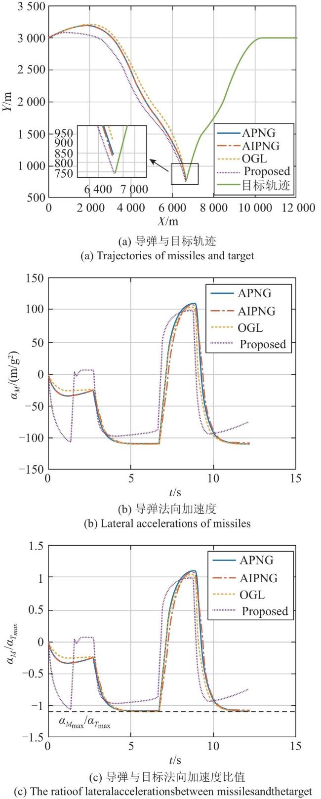
为保证在同等条件下进行对比,取N_APNG=4,N_AIPNG=4。式(99),(101)中接近速度V_c=-

$\stackrel{\mathit{　}·}{\mathit{r}}$

。对比仿真结果如表3和图7所示。

表3 脱靶量对比

Table 3 Miss distance comparison

制导律	脱靶量/m
APNG	83.79
AIPNG	67.69
OGL	160.69
Proposed	0.85

显示原图|下载原图ZIP|生成PPT

图7 对比仿真结果

Fig.7 Simulation results with comparison

观察对比仿真结果,表2和图7(a)表明四种制导律中,仅有本文所提最优制导律能够拦截目标,APNG、AIPNG、OGL三种制导律均脱靶。观察图7(b)-(c)可知,造成脱靶的原因是APNG、AIPNG及OGL在拦截末端法向过载均处于饱和状态,末端过载裕量极小。而本文所提最优制导律的末端过载未饱和,且整个第二阶段内过载比均小于1。这种现象是由于APNG在设计过程中假设目标执行常值机动,因此对目标机动的补偿不准确;AIPNG虽对目标机动进行了精确补偿,但未考虑导弹和目标内回路延迟的影响,过载指令延迟导致脱靶量未被及时补偿;OGL仅对导弹的内回路延迟进行了补偿,但未对目标的内回路延迟进行补偿。因此,本文所提最优制导律在拦截机动目标时更具优势。

4 结论

本文针对均势机动目标的拦截问题,设计了一种两阶段最优制导控制一体化方法。通过引入相对参考坐标系进行建模,对目标过载进行实时精确补偿,避免过补偿或欠补偿导致的额外过载消耗。第一阶段制导律能在最短距离内消除初始指向误差,并满足均势拦截条件。第二阶段引入导弹和目标的内回路延迟,进行制导控制一体化设计,以最小能量消耗抵消目标机动,并实时补偿内回路延迟的影响,实现该阶段内弹目过载比始终小于1。在不同初始速度倾角条件下,该制导律均能精确拦截目标,并保证末端过载比小于1。仿真结果表明,与APNG、AIPNG和OGL相比,在导弹与目标过载能力相近的条件下,本文所提制导律需用弹目过载比低,可精准拦截目标;而其余三种制导律皆因末端过载饱和而导致脱靶量显著增大。

参考文献

原文顺序 | 文献年度倒序 | 文中引用次数倒序

[1]

张紫琪, 宋天威, 王楷, 等. 拦截高速机动目标的终端视线角约束三维末制导律设计[J]. 弹箭与制导学报, 2025, 45(6):986-994.

ZHANG

Z Q

, SONG

T W

, WANG

, et al. Design of three-dimensional terminal guidance law with terminal line-of-sight angle constraints for intercepting high-speed maneuvering targets[J]. Journal of Projectiles,Rockets,Missiles and Guidance, 2025, 45(6):986-994.

[2]	方东洋, 鲍俊龙, 吴光辉, 等. 考虑导引头探测角度控制的直接碰撞拦截末制导律设计[J]. 弹箭与制导学报, 2024, 44(4):89-93. DOI FANG D Y, BAO J L, WU G H, et al. Terminal guidance for hit-to-kill interception with detection angle control[J]. Journal of Projectiles,Rockets,Missiles and Guidance, 2024, 44(4):89-93.

[3]	任淼, 刘晶晶, 文琳. 2021年国外空空导弹发展动态研究[J]. 航空兵器, 2022, 29(4):33-41. REN M, LIU J J, WEN L. Research on foreign air-to-air missiles’ development in 2021[J]. Aero Weaponry, 2022, 29(4):33-41.

[4]	马寒冰, 贾晓洪, 徐琰珂, 等. 基于FAHP-熵权-TOPSIS模型的空空导弹制导律评估[J]. 弹箭与制导学报, 2025, 45(3):359-365. MA H B, JIA X H, XU Y K, et al. Research on guidance law based on FAHP-entropy weight-TOPSIS integrated evaluation method[J]. Journal of Projectiles,Rockets,Missiles and Guidance, 2025, 45(3):359-365.

[5]	王龙, 李斌. 基于非线性规划的中近距空空导弹增程弹道设计方法[J]. 弹箭与制导学报, 2021, 41(6):76-81. DOI WANG L, LI B. Trajectory design for extending range of medium and short range air-to-air missiles based on non-linear programming[J]. Journal of Projectiles,Rockets,Missiles and Guidance, 2021, 41(6):76-81.

[6]	TEKIN R, ERER K S. Impact time and angle control against moving targets with look angle shaping[J]. Journal of Guidance,Control,and Dynamics, 2020, 43(5):1020-1025. DOI

[7]	李波, 范盘龙, 李卿莹, 等. 一种综合优势下的空空导弹接力制导混合优化方法[J]. 宇航学报, 2019, 40(2):191-198. LI B, FAN P L, LI Q Y, et al. A hybrid optimization method of air-to-air missile relay guidance based on integrated superiority[J]. Journal of Astronautics, 2019, 40(2):191-198.

[8]	BRYSON A E. Applied optimal control:optimization,estimation and control[M]. New York,USA: Taylor & Francis,1975:1-110.

[9]	HE S M, LEE C H. Optimality of error dynamics in missile guidance problems[J]. Journal of Guidance,Control,and Dynamics, 2018, 41(7):1624-1633. DOI

[10]	HE S M, LEE C H. Optimal proportional-integral guidance with reduced sensitivity to target maneuvers[J]. IEEE Transactions on Aerospace and Electronic Systems, 2018, 54(5):2568-2579. DOI

[11]	LI H Y, WANG J, HE S M, et al. Nonlinear optimal impact-angle-constrained guidance with large initial heading error[J]. Journal of Guidance,Control,and Dynamics, 2021, 44(9):1663-1676. DOI

[12]	CHAI R Q, TSOURDOS A, SAVVARIS A, et al. Review of advanced guidance and control algorithms for space/aerospace vehicles[J]. Progress in Aerospace Sciences, 2021, 122:100696. DOI

[13]	SONG J H, SONG S M. Three-dimensional guidance law based on adaptive integral sliding mode control[J]. Chinese Journal of Aeronautics, 2016, 29(1):202-214. DOI

[14]	KADA B. Arbitrary-order sliding-mode-based homing-missile guidance for intercepting highly maneuverable targets[J]. Journal of Guidance,Control,and Dynamics, 2014, 37(6):1999-2013. DOI

[15]	CHO D, KIM H J, TAHK M J. Fast adaptive guidance against highly maneuvering targets[J]. IEEE Transactions on Aerospace and Electronic Systems, 2016, 52(2):671-680. DOI

[16]	王思卓, 范世鹏, 林德福, 等. 考虑目标机动和落角约束的二阶滑模制导律[J]. 兵工学报, 2022, 43(12):3048-3061. WANG S Z, FAN S P, LIN D F, et al. Second order sliding mode guidance law considering target maneuver and impact angle constraint[J]. Acta Armamentarii, 2022, 43(12):3048-3061. DOI

[17]	LI C Y, JING W X, WANG H, et al. Gain-varying guidance algorithm using differential geometric guidance command[J]. IEEE Transactions on Aerospace and Electronic Systems, 2010, 46(2):725-736. DOI

[18]	YE J K, LEI H M, XUE D F, et al. Nonlinear differential geometric guidance for maneuvering target[J]. Journal of Systems Engineering and Electronics, 2012, 23(5):752-760. DOI

[19]	LEE C H, SEO M G. Newinsights into guidance laws with terminal angle constraints[J]. Journal of Guidance,Control,and Dynamics, 2018, 41(8):1832-1837. DOI

[20]	WANG J, WANG Y H, LI H Y, et al. Analytical optimal counter guidance against proportional navigation[J]. Journal of Guidance,Control,and Dynamics, 2024, 47(12):2631-2640. DOI

[21]	ZARCHAN P. Tactical and strategic missile guidance[M]. 6th ed.Reston, VA, USA:AIAA,2012:21-22.

[22]	韩京清. 自抗扰控制技术[M]. 北京: 国防工业出版社,2008:49-66. HAN J Q. Active disturbance rejection control technique[M]. Beijing: National Defense University Press,2008:49-66.

[23]	WANG Y H, WANG J, FAN S P. Parameter identification of a PN-guided incoming missile using an improved multiple-model mechanism[J]. IEEE Transactions on Aerospace and Electronic Systems, 2023, 59(5):5888-5899.

Options

文章导航

模态框（Modal）标题

摘要

本文引用格式

Abstract

0 引言

1 问题描述

1.1 纵向平面交战几何关系

图1 纵向平面交战几何示意图

1.2 相对参考系下的运动关系

图2 参考系下的相对运动关系

2 最优制导律设计

2.1 均势拦截的必要条件

2.2 制导律设计

图3 线性化相对参考坐标系

3 仿真验证

表1 仿真初始条件

图4 拦截bang-bang机动目标的仿真结果

图5 不同辨识误差下的仿真结果

图6 不同辨识误差下的脱靶量

表2 不同辨识误差下的命中率

表3 脱靶量对比

图7 对比仿真结果

4 结论

参考文献